Stop Guessing. Build a Real Estate Forecast Engine.
Forecasting real estate trends with a BI tool is not about dragging and dropping a few widgets. It’s about forcing dirty, disconnected data into a structure that can be modeled. The reports are the last, easiest part of the job. The real work is in the plumbing, the data shaping, and the logic-checks that prevent you from presenting total fiction to people who make expensive decisions.
Most forecasting projects fail at the data source. You think you have a clean feed until you discover one county provides assessed value and another provides market value, and neither of them label it correctly. This guide is about building the data pipeline first, then letting the BI tool do its simple arithmetic.
Prerequisites: The Non-Negotiable Toolkit
Before writing a single line of code, you need to assemble your sources and tools. Skipping this step means you will inevitably rebuild your entire data model three weeks into the project after discovering a critical source you ignored.
- BI Platform: Power BI or Tableau. Power BI is cheaper if you’re already in the Microsoft ecosystem. Tableau is more flexible with certain data sources but is a definite wallet-drainer. Either will work. Don’t use some lightweight, browser-only tool. You need horsepower for data modeling.
- Data Warehouse: A centralized repository is mandatory. Snowflake, BigQuery, or Redshift are the typical choices. Attempting to connect your BI tool directly to a dozen different flat files and raw API feeds is a direct path to a sluggish, unmanageable dashboard that times out on every query.
- Scripting Language: Python. The Pandas and Requests libraries are your workhorses for data extraction and cleaning. Nothing else offers this combination of power and community support for data manipulation.
- API Keys: You need programmatic access to data. Get keys for a real estate marketplace like Zillow or Redfin, government sources like the U.S. Census Bureau for demographic data, and possibly a local MLS feed if you can get authorized access. Prepare for rate limits and poorly documented endpoints.
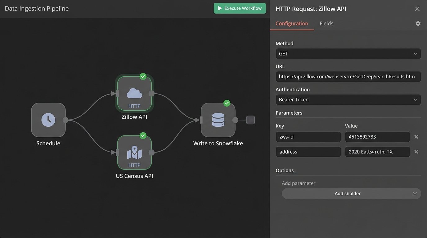
Step 1: Ingesting the Raw Feeds
The goal here is data acquisition, not data perfection. We pull everything into a staging area within our data warehouse. This is a raw data dump. We want to get the data out of its original, fragile source and into an environment we control as quickly as possible. We are not transforming anything yet. We are just landing the planes.
A common failure is to try and clean the data on the fly during ingestion. This couples your extraction script to the data’s current state. When an API provider decides to change a field name from `listing_price` to `price_listed_usd` without notice, your entire pipeline breaks. Ingest first, then apply transformations in a separate, controlled process.
Set up scheduled jobs, probably using Airflow or a simple cron job running a Python script, to hit these APIs. Stagger your API calls to avoid hitting rate limits. A 429 “Too Many Requests” error at 2 AM is a problem you don’t need.
This process is about building a local copy of the external world’s data. It’s your source of truth, even if that truth is messy. Trying to bridge dozens of external data sources directly in a BI tool is like trying to shove a firehose through a needle. You are forcing a visualization tool to do the heavy lifting of a dedicated ETL process, and it will choke.
Step 2: The Brutal Reality of Data Cleaning
Your raw data is garbage. Accept it. Prices will be stored as strings with dollar signs. Addresses will be inconsistent. Key metrics like square footage will be null. This is where the majority of your time will be spent. We use Python scripts to systematically strip, standardize, and impute this data before it ever touches the core tables of our warehouse.
Focus on creating a single, consistent schema. All addresses must be broken down into the same components: street number, street name, city, state, zip. All prices must be converted to a numeric type. All dates must be forced into ISO 8601 format (`YYYY-MM-DD`).
Here is a dead-simple Python function using Pandas to illustrate the point. It handles one of the most common data quality problems: non-numeric price fields.
import pandas as pd

import numpy as np
def clean_price_data(df, column_name='price'):
"""
Strips non-numeric characters from a price column and converts to float.
Handles common junk data like '$', ',', and 'Call for Price'.
"""
if column_name not in df.columns:
print(f"Error: Column '{column_name}' not found.")
return df
# Force the column to be a string to use string methods
df[column_name] = df[column_name].astype(str)
# Replace non-numeric patterns. The regex handles '$' and ','
df[column_name] = df[column_name].str.replace(r'[$,]', '', regex=True)
# Convert to numeric, coercing errors to NaN (Not a Number)
# This catches strings like 'Call for Price' or empty fields
df[column_name] = pd.to_numeric(df[column_name], errors='coerce')
# Optional: Fill NaN values with a specific value, like the median or 0
# For forecasting, leaving it as NaN might be better to signal missing data
# median_price = df[column_name].median()
# df[column_name].fillna(median_price, inplace=True)
return df
This single function is more resilient than anything you can build with a graphical interface in a BI tool. Apply this kind of logic systematically to every single column you plan to use.
Don’t just delete rows with missing data. That’s the lazy way out and it will bias your dataset. If square footage is missing for 10% of your properties, find out why. Maybe it’s a specific property type, like vacant land, that is skewing your analysis. Isolate the problem before you delete the evidence.
Step 3: Engineering Features That Matter
Raw data rarely contains the most predictive signals. We have to create them. Feature engineering is the process of using domain knowledge to transform raw data into features that better represent the underlying problem for machine learning models or statistical analysis.
This is where SQL becomes critical. Working on your clean data inside the warehouse, you can write queries to generate new, high-value columns. You are building the levers that your forecasting model will pull.
- Price Per Square Foot: A fundamental valuation metric. `sale_price / square_footage`.
- Days On Market: A key indicator of market velocity. `date_sold – date_listed`.
- Rolling Averages: Smooth out short-term volatility. Calculate the 30, 90, and 180-day average sale price for each zip code.
- Proximity to Amenities: Using geospatial functions, calculate the distance from each property to the nearest school, park, or public transit stop. This requires another data source but adds significant predictive power.
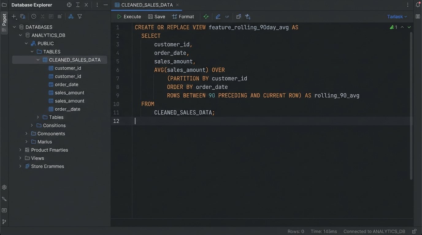
A SQL query to generate a rolling 90-day average sale price by postal code looks something like this. This is impossible to do efficiently inside the BI tool itself, but trivial inside a proper data warehouse.
CREATE OR REPLACE VIEW V_PROPERTY_ANALYTICS AS

SELECT

    property_id,

    sale_date,

    sale_price,

    postal_code,

    AVG(sale_price) OVER (

        PARTITION BY postal_code

        ORDER BY sale_date

        ROWS BETWEEN 90 PRECEDING AND CURRENT ROW

    ) AS avg_price_90_day_rolling

FROM

    CLEANED_SALES_DATA;
By creating this as a view or a materialized table, the heavy computation is done once in the database. The BI tool just has to query a pre-calculated column. It is fast, efficient, and scalable.
Step 4: Connecting the BI Tool
With a clean, feature-rich table in your warehouse, connecting it to Power BI or Tableau is the easy part. You have two main choices for connection type: Import or DirectQuery.
Import Mode: The BI tool pulls a copy of your data and stores it in its own internal, highly compressed columnar database (VertiPaq for Power BI, Hyper for Tableau). Queries are lightning fast because the data is in-memory. The downside is that data is only as fresh as your last scheduled refresh. This is the correct choice for 95% of forecasting use cases.
DirectQuery Mode: The BI tool sends live queries to your data warehouse every time a user interacts with a visual. The data is always current, but performance is entirely dependent on your warehouse’s speed and the complexity of the query. It’s also much harder on the source system. Use this only if you have a legitimate, hard requirement for real-time data, which for trend forecasting, you almost never do.
Connect to the views and tables you built in Step 3. Do not connect to the raw, staged data. The BI tool’s data model should be simple and clean, reflecting the work you already did. You are not performing complex transformations here. You are just building relationships between your clean tables.
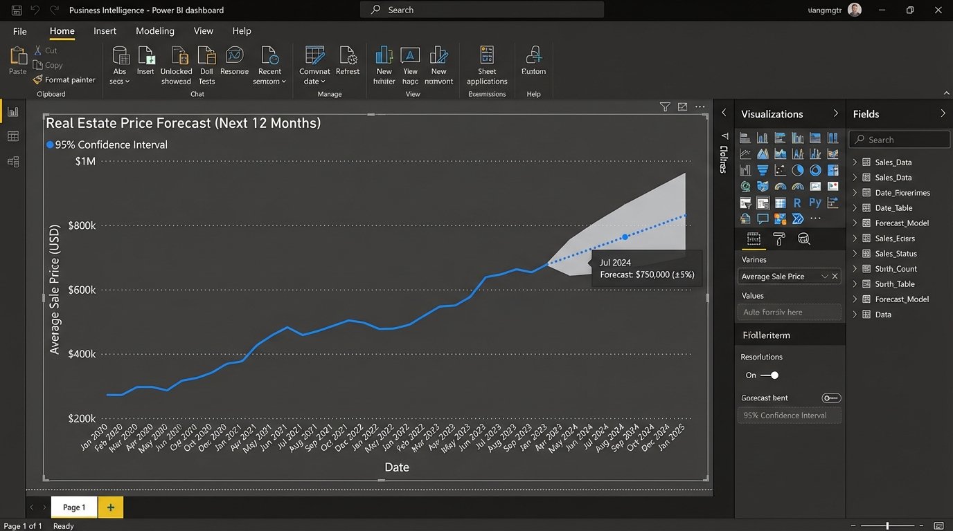
Step 5: Forecasting Inside the Tool
BI tools have built-in forecasting functions. They are typically based on models like exponential smoothing (ETS). These are not complex, deep learning models. They are statistical workhorses designed to extrapolate time-series data. They work by decomposing the historical data into three components: level, trend, and seasonality.
In your BI tool, you will typically drag your date field and your target metric (e.g., `avg_price_90_day_rolling`) onto a line chart. From there, you can access the analytics pane and add a forecast. You can configure the forecast length (how many periods to predict) and the confidence interval (the probability that the true value will fall within the predicted range). A 95% confidence interval is standard.
These models are a black box. You feed them a clean time series, and they produce a forecast. Their main limitation is that they are univariate, meaning they only consider the past values of the metric itself to predict its future. They do not natively incorporate the other features you engineered, like “days on market” or economic indicators. For a more advanced forecast that considers multiple input variables (a multivariate model), you need to step outside the BI tool and use a Python or R model, then import the results back in.
Step 6: Validation and Not Lying to Yourself
A forecast is useless if you can’t measure its accuracy. The simplest method is backtesting. Pretend it’s one year ago. Feed your model data only up to that point and ask it to forecast the next 12 months. Now, compare that forecast to what actually happened in the real-world data you have.
Calculate standard accuracy metrics like Mean Absolute Error (MAE) or Root Mean Square Error (RMSE). This gives you a concrete number for how far off your model is, on average. This number is critical. It grounds your pretty forecast chart in reality and gives your audience a sense of the model’s reliability.
A forecast is not a promise. It is a probabilistic assessment based on historical patterns. Your job is to show the patterns, run the numbers, and clearly communicate the model’s margin of error. Anything less is just drawing lines on a chart and hoping for the best.